Figures S17-S28: Longitudinal strain rate analysis for all tests
Contents
Figures S17-S28: Longitudinal strain rate analysis for all tests
This notebooks shows the analysis of longitudinal strain rate (abbreviated as LSR in Table S2) with the supplemental figures in the bottom.
Basic information, importing modules, load data list and flow-area shapefile
See Table S1 for all the Kaskawulsh glacier images and parameter sets used in this study.
import glaft
import matplotlib as mpl
import matplotlib.pyplot as plt
import pandas as pd
from cmcrameri import cm as cramericm
We start by loading the data list. Whichever line in the cell blow works for reproducing the figures.
../manifest.csvcontains only the parameter table (Table S1)../results_2022.csvcontains both the parameter table and all the metrics calculated (Table S2) in this study.
If you want to reproduce the workflow and the figures, make sure you have downloaded all necessary input files from https://doi.org/10.17605/OSF.IO/HE7YR and have updated the Vx and Vy columns in either csv file with the downloaded file paths before starting the analysis.
# df = pd.read_csv('../manifest.csv', dtype=str)
df = pd.read_csv('../results_2022.csv', dtype=str)
Specify flow area. Change the path to the downloaded shapefile from https://doi.org/10.17605/OSF.IO/HE7YR before running the cell.
in_shp = '/home/jovyan/Projects/PX_comparison/shapefiles/glacier_V1_Kaskawulsh_s_inwardBuffer600m.shp'
Perform analysis
exps = {}

for idx, row in df.iterrows():
    exp = glaft.Velocity(vxfile=row.Vx, vyfile=row.Vy, on_ice_area=in_shp, kde_gridsize=60, thres_sigma=2.0)
    exp.longitudinal_shear_analysis()
    exps[idx] = exp
Visualize results
3.1. Distribution of longitudinal strain rate
Click to show
# Font and line width settings
font = {'size' : 13}
mpl.rc('font', **font)
axes_settings = {'linewidth' : 2}
mpl.rc('axes', **axes_settings)
def plot_batch(sub_df, zoom=False, datestr=''):
"""
Plot longitudinal strain rate distribution for all the tests from the same image pair.
"""
fig, axs = plt.subplots(8, 6, figsize=(20, 26), constrained_layout=True)
n = 0
for idx, row in sub_df.iterrows():
ax_sel = axs[n // 6, n % 6]
exp = exps[idx]
if zoom:
exp.plot_zoomed_extent(ax=ax_sel, metric=2)
ax_sel.set_xlim(-0.15, 0.15)
ax_sel.set_ylim(-0.15, 0.15)
else:
exp.plot_full_extent(ax=ax_sel, metric=2)
# adjust extent
xmin, xmax = ax_sel.get_xlim()
ymin, ymax = ax_sel.get_ylim()
newmin = max(min(xmin, ymin), -10)
newmax = min(max(xmax, ymax), 10)
ax_sel.set_xlim(newmin, newmax)
ax_sel.set_ylim(newmin, newmax)
ax_sel.set_aspect('equal', adjustable='box')
# show incorrect match percentage
ax_sel.text(0.95, 0.95, '{:.1f}%'.format(exp.outlier_percent * 100), ha='right', va='top', transform=ax_sel.transAxes, backgroundcolor=(1, 1, 1, 0.5))
#### title label
templatesize = row['Template size (px)']
# change long GIV label "varying: multi-pass" to "multi"
templatesize = 'multi' if templatesize == 'varying: multi-pass' else templatesize
if row.Software == 'Vmap':
label = '-'.join((row.Software, templatesize, row['Pixel spacing (px)'], row.Prefilter)) + '\n' + row.Subpixel
else:
label = '-'.join((row.Software, templatesize, row['Pixel spacing (px)'], row.Prefilter))
ax_sel.set_title(label)
####
n += 1
# delete empty axes
for i in range(n, 48):
ax_sel = axs[i // 6, i % 6]
fig.delaxes(ax_sel)
# legends
fig.text(0.5, 0.06,
"{}".format(datestr) + "\nX axis: normal strain rate $\dot{\epsilon}_{x'x'}$ (day$^{-1}$) \nY axis: shear strain rate $\dot{\epsilon}_{x'y'}$ (day$^{-1}$) \nPercentage: amount of pixels falling outside of the red box to all pixels",
fontsize=16, ha='center')
return fig, axs
Click to show
### To reproduce the figures, uncomment and run the rest of this cell.

# for datestr in ['LS8-20180304-20180405', 'LS8-20180802-20180818', 'Sen2-20180304-20180314', 'Sen2-20180508-20180627']:
#     sub_df = df.loc[df['Date'] == datestr]
#     fig, axs = plot_batch(sub_df, zoom=False, datestr=datestr)
#     fig.patch.set_facecolor('xkcd:white')
#     fig.savefig('figs/{}-LSR-full.png'.format(datestr))
#     fig, axs = plot_batch(sub_df, zoom=True, datestr=datestr)
#     fig.patch.set_facecolor('xkcd:white')
#     fig.savefig('figs/{}-LSR-zoomed.png'.format(datestr))
 Figure S17. Longitudinal strain rate distribution of the pair
 LS8-20180304-20180405 (full extent).
 Figure S18. Longitudinal strain rate distribution of the pair
 LS8-20180304-20180405 (zoomed with kernel density estimation).
 Figure S19. Longitudinal strain rate distribution of the pair
 LS8-20180802-20180818. (full extent).
 Figure S20. Longitudinal strain rate distribution of the pair
 LS8-20180802-20180818. (zoomed with kernel density estimation).
 Figure S21. Longitudinal strain rate distribution of the pair
 Sen2-20180304-20180314. (full extent).
 Figure S22. Longitudinal strain rate distribution of the pair
 Sen2-20180304-20180314. (zoomed with kernel density estimation).
 Figure S23. Longitudinal strain rate distribution of the pair
 Sen2-20180508-20180627. (full extent).
 Figure S24. Longitudinal strain rate distribution of the pair
 Sen2-20180508-20180627. (zoomed with kernel density estimation).
3.2. Map of longitudinal strain rate
Click to show
def plot_batch_strainrate(sub_df, vmax=0.03, datestr=''):
    """
    Plot longitudinal strain rate map for all the tests from the same image pair.
    """
    fig, axs = plt.subplots(8, 6, figsize=(20, 20), constrained_layout=True)
    n = 0

    for idx, row in sub_df.iterrows():

        ax_sel = axs[n // 6, n % 6]
        exp = exps[idx]

        mappable_strain = exp.plot_strain_map(ax=ax_sel, vmax=vmax, base_colormap=cramericm.tokyo)
        ax_sel.set_aspect('equal', adjustable='datalim')

        #### title label
        templatesize = row['Template size (px)']
        # change long GIV label "varying: multi-pass" to "multi"
        templatesize = 'multi' if templatesize == 'varying: multi-pass' else templatesize
        if row.Software == 'Vmap':
            label = '-'.join((row.Software, templatesize, row['Pixel spacing (px)'], row.Prefilter)) + '\n' + row.Subpixel
        else:
            label = '-'.join((row.Software, templatesize, row['Pixel spacing (px)'], row.Prefilter))
        ax_sel.set_title(label)
        ####

        n += 1

    # delete empty axes
    for i in range(n, 48):
        ax_sel = axs[i // 6, i % 6]
        fig.delaxes(ax_sel)

    # legends (colorbar)
    strain_cmap_label = "$\sqrt{\dot{\epsilon}_{x'x'}^2 + \dot{\epsilon}_{x'y'}^2}$ (1/day)"
    cbar_label = datestr + '\n' + strain_cmap_label
    cax = fig.add_axes([0.2, 0.09, 0.17, 0.017])

    fig.colorbar(mappable_strain, cax=cax, orientation='horizontal', label=cbar_label)

    return fig, axs
Click to show
### To reproduce the figures, uncomment and run the rest of this cell.

# for datestr in ['LS8-20180304-20180405', 'LS8-20180802-20180818', 'Sen2-20180304-20180314', 'Sen2-20180508-20180627']:
#     sub_df = df.loc[df['Date'] == datestr]
#     fig, axs = plot_batch_strainrate(sub_df, datestr=datestr)
#     fig.patch.set_facecolor('xkcd:white')
#     fig.savefig('figs/{}-LSR-map.png'.format(datestr))
 Figure S25. Longitudinal strain rate map of the pair
 LS8-20180304-20180405 full extent).
 Figure S26. Longitudinal strain rate map of the pair
 LS8-20180802-20180818. full extent).
 Figure S27. Longitudinal strain rate map of the pair
 Sen2-20180304-20180314. full extent).
 Figure S28. Longitudinal strain rate map of the pair
 Sen2-20180508-20180627. full extent).
Save results
for idx, exp in exps.items():
    df.loc[idx, 'LSR-uncertainty-nm'] = exp.metric_alongflow_normal
    df.loc[idx, 'LSR-uncertainty-sh'] = exp.metric_alongflow_shear

df.to_csv('../results_2022.csv', index=False)