Reference
Contents
Reference
glaft.Velocity class
       glaft.Velocity(vxfile:


       str=None,


       vyfile:


       str=None,


       wfile:


       str=None,


       static_area:


       str=None,


       on_ice_area:


       str=None,


       nodata:


       float=-9999.0,


       velocity_unit:


       str='m/day',


       thres_sigma:


       float=2.0,


       kde_gridsize:


       int=60)
Construct an experiment to calculate velocity map benchmarking metrics.
vxfile: str, Vx raster file path
(single band with meters as the geotransform unit)
vyfile: str, Vy raster file path
(single band with meters as the geotransform unit)
wfile: str, weight raster file path [Optional]
static_area: str, static area (shapefile) file path
on_ice_area: str, on-ice area (shapefile) file path
nodata: float, nodata value in the provided geotiff. NOT FULLY IMPLEMENTED YET.
velocity_unit: str, velocity unit to be shown on the result plots.
thres_sigma: float, selected thresholding z values.
kde_gridsize: int, grid size used for evaluating a crude KDE surface
(larger value means a faster but less precise process)
         Velocity.static_terrain_analysis(plot=None,


         ax=None)
Perform the static terrain analysis and calculate the correct-match uncertainty.
plot: None for no plot;
"full" for plotting the results in the full extent;
"zoomed" for plotting the results in the zoomed extent.
ax: matplotlib.axes object to place the plot.
         Velocity.longitudinal_shear_analysis(plot=None,


         ax=None)
Perform the longitudinal strain rate analysis and calculate the associated metrics.
plot: None for no plot;
"full" for plotting the results in the full extent;
"zoomed" for plotting the results in the zoomed extent.
ax: matplotlib.axes object to place the plot.
         Velocity.plot_full_extent(ax=None,


         rect=None,


         metric:


         int=1,


         **pt_style)
Plot the analysis results in the full extent.
ax: matplotlib.axes object to place the plot.
rect: style of the rectanglar box indicating the correct match area.
If None, the plot uses thick red line as default.
See Velocity.create_rectangle_patch for details.
metric: which metric to be plotted.
1 for static terrain;
2 for along-flow strain rate.
pt_style: point style passed to plt.scatter.
         Velocity.plot_zoomed_extent(ax=None,


         rect=None,


         base_colormap=None,


         metric:


         int=1,


         **pt_style)
Plot the analysis results in the zoomed extent focusing on the correct-match area.
ax: matplotlib.axes object to place the plot.
rect: style of the rectanglar box indicating the correct match area.
If None, the plot uses thick red line as default.
See Velocity.create_rectangle_patch for details.
base_colormap: colormap for showing the KDE probability distribtuion.
If None, the default (cramericm.bamako_r) is used.
metric: which metric to be plotted.
1 for static terrain;
2 for along-flow strain rate.
pt_style: point style passed to plt.scatter.
         Velocity.create_rectangle_patch(var_x,


         var_y,


         **rect_style)
Create a rectangle patch to be plotted on the visualization of the processing results.
var_x: half width of the rectangle
var_y: half height of the rectangle
rect_style: style of the rectangle.
Default is {'linewidth': 2, 'edgecolor': 'xkcd:cranberry',
'facecolor': 'none', 'alpha': 0.7}
Returns
--------------
matplotlib.patches.Rectangle object.
         Velocity.plot_strain_map(ax=None,


         base_colormap=None,


         vmax=None)
Show the strain map. Only works after longitudinal_shear_analysis is performed).
ax: matplotlib.axes object to place the plot.
base_colormap: colormap for showing the strain map.
If None, the default (cramericm.bamako) is used.
vmax: value at where color is saturated.
If None, the saturation limit will be automatically determined.
Velocity.cal_invalid_pixel_percent()
Calculate the amount of invalid pixels in a velocity map.
Important attributes
Velocity.vxfileVx file path.Velocity.vyfileVy file path.Velocity.wfileWeight file path.Velocity.static_areastatic area geometries file path.Velocity.on_ice_areaon-ice area geometries file path.Velocity.nodataNoData value for the raster files.Velocity.velocity_unitvelocity unit to be shown on the result plots.Velocity.vx2-D, clipped vx dataVelocity.vy2-D, clipped vy dataVelocity.xy= np.vstack([flattened_vx, flattened_vy]) –> (1-D)-by-2 array containing vx and vy.Velocity.w2-D, clipped weight dataVelocity.w_flat1-D, clipped & flattened weight dataVelocity.dxvelocity map pixel spacing, xVelocity.dyvelocity map pixel spacing, yVelocity.thres_sigmaselected thresholding z values.Velocity.kernelKDE kernel (defaultepanechnikov)Velocity.bandwidthKDE bandwidth (default: calculated using the rule of thumb)Velocity.kde_gridsizegrid size used for evaluating a crude KDE surface (larger value means a faster but less precise process)Velocity.mesh_fineFinal KDE meshVelocity.mesh_fine_zKDE values at the final KDE mesh verticesVelocity.mesh_fine_thres_idxboolean array showing whether a vertex falls within the correct match areaVelocity.metric_static_terrain_xdelta_xVelocity.metric_static_terrain_ydelta_yVelocity.kdepeak_xKDE peak location xVelocity.kdepeak_yKDE peak location yVelocity.outlier_percentIncorrect match percentage (*100%)Velocity.invalid_percentInvalid pixels percentage (*100%)Velocity.flow_thetaFlow directionVelocity.exxnormal strain rate exx, image axisVelocity.eyynormal strain rate eyy, image axisVelocity.exyshear strain rate exy, image axisVelocity.flow_exxnormal strain rate exx, flow axis (that is, ex’x’)Velocity.flow_eyynormal strain rate eyy, flow axis (that is, ey’y’)Velocity.flow_exyshear strain rate exy, flow axis (that is, ex’y’)Velocity.metric_alongflow_normaldelta_x’x’Velocity.metric_alongflow_sheardelta_x’y’
Auxillary functions
       glaft.show_velocomp(gtiff:


       str,


       ax=None,


       **cm_settings)
Preview a geotiff file (presuming a velocity map).
Parameters
-------------
gtiff: geotiff file path (much be single band. e.g., Velocity component, such as Vx)
ax: matplotlib.axes object to place the plot
cm_settings: colormap settings to be used in the visualization.
Default: {'vmin': -2, 'vmax': 2, 'cmap': cramericm.broc_r}
Returns
--------------
cm_settings: colormap settings using in the visualization.
       glaft.prep_colorbar_mappable(vmin=-2,


       vmax=2,


       cmap=cramericm.broc_r)
Generate a mappbale object for creating a colorbar.
Parameters
-------------
vmin: colormap lower range
vmax: colormap upper range
cmap: colormap object as the master colormap

Returns
--------------
mappable: matplotlib.mappable object
glaft.naof2(im)
NAOF preprocessing filter. Translated to Python from the GIV source code. All implementation credit to Max VWDV.
MaxVWDV. (2021). MaxVWDV/glacier-image-velocimetry: Glacie Image Velocimetry (v1.0.1). Zenodo. https://doi.org/10.5281/zenodo.4904544
Parameters
-------------
im:       np.ma.array;  input image

Returns
--------------
naof_im:  np.ma.array;  image with NAOF filter applied